Following Quadratic Programming with R, this is another example of how to solve quadratic programming problem with R package “quadprog“.

Why Another Example?

“quadprog” package requires us to rewrite the quadratic equation in the proper matrix equation as above. You may have the following questions:

• What if our equation is to maximize the objective function instead of minimize it?
• What if the inequality constraints are “less than (<=)” instead of “more than (>=)”?
• What if there is no equality constraints?
• …

To give you an idea how to answer these questions, this post will give you another example.

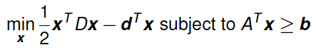
Example

Be aware that this problem is to maximize the objective function and the first two inequality constraints are in “<=” form.

Therefore, we have to rewrite it as follows:

Minimize P = x₁² + x₂² – 5x₁ – 7x₂ + 5, subject to:

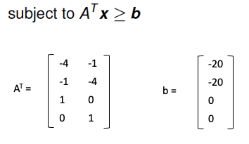
– 4x₁ – x₂ >= – 20

– x₁ – 4x₂ >= – 20

x₁ >= 0

x₂ >= 0

Matrix Notation

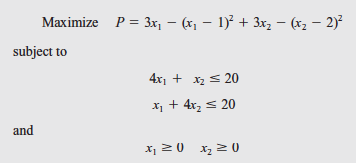
First, consider the matrix notation for a general quadratic function of two variables: x₁ and x₂:

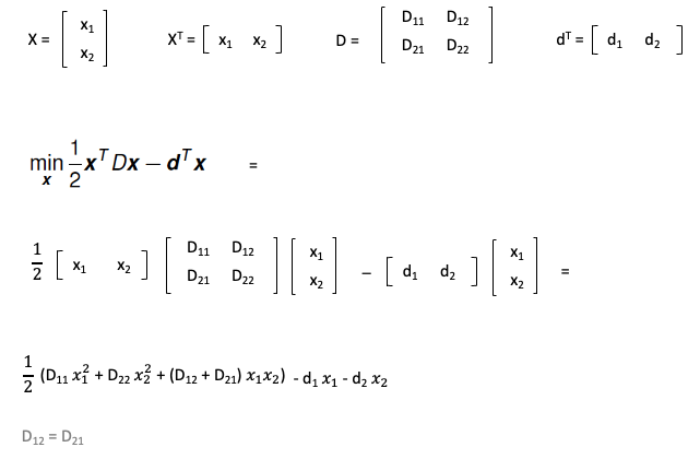
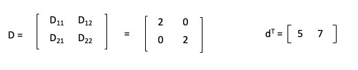
Second, we can extract the matrix D and vector d by parameter mapping to our example:

Similarly, the constraint matrix A^T and the vector b can be found:

R Code & Output

solve.QP(Dmat, dvec, Amat, bvec, meq=0, factorized=FALSE)

- Dmat    
matrix appearing in the quadratic function to be minimized.

- dvec    
vector appearing in the quadratic function to be minimized.

- Amat    
matrix defining the constraints under which we want to minimize the quadratic function.

- bvec    
vector holding the values of b_0 (defaults to zero).

- meq    
the first meq constraints are treated as equality constraints, all further as inequality constraints (defaults to 0).

- factorized    
logical flag: if TRUE, then we are passing R^(-1) (where D = R^T R) instead of the matrix D in the argument Dmat.

# Load "quadprog" package
# library(quadprog)

# Matrix appearing in the quadratic function
Dmat <- matrix(c(2, 0, 0, 2), nrow = 2)

# Vector appearing in the quadratic function
dvec <- c(5, 7)

# Matrix defining the constraints
Amat <- t(matrix(c(-4, -1, 1, 0, -1, -4, 0, 1), nrow = 4))

# Vector holding the value of b_0
bvec <- c(-20, -20, 0, 0)

# meq indicates how many constraints are equality 
# No constraint is equality in this example, so meq = 0 (by default)
qp <- solve.QP(Dmat, dvec, Amat, bvec)
qp

$solution
[1] 2.5 3.5

$value
[1] -18.5

$unconstrained.solution
[1] 2.5 3.5

$iterations
[1] 1 0

$Lagrangian
[1] 0 0 0 0

$iact
[1] 0

Therefore, when x₁ = 2.5 and x₂ = 3.5 the quadratic function is minimized (-18.5 + 5 = -13.5, don’t forget the constant 5). However, since we rewrited the objective function at the beginning, we have to interpret the results accordingly. In other words, in order to maximize the original quadratic function, we choose x₁ = 2.5 and x₂ = 3.5. Further more, the maximized values is 13.5.