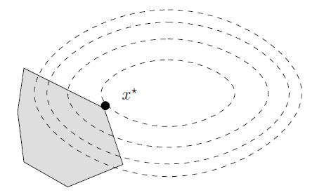
Quadratic programming problems can be solved with “quadprog” package in R and the key point is to find the matrix notation of quadratic programming problems:

Example

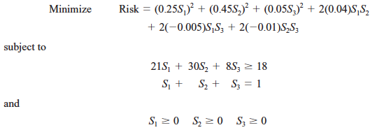
Let’s figure out how to do it with an example of “Applying Nonlinear Programming to Portfolio Selection”:

Please note that, this example involves three variables (x₁, x₂, and x₃). If you want an example of two variables (x₁ and x₂), please check my another post: Another Quadratic Programming Example with R.

“It now is common practice for professional managers of large stock portfolios to use computer models based partially on nonlinear programming to guide them. Because investors are concerned about both the expected return (gain) and the risk associated with their investments, nonlinear programming is used to determine a portfolio that, under certain assumptions, provides an optimal trade-off between these two factors.”

Frederick & Mark (2014, p.283)

Matrix Notation

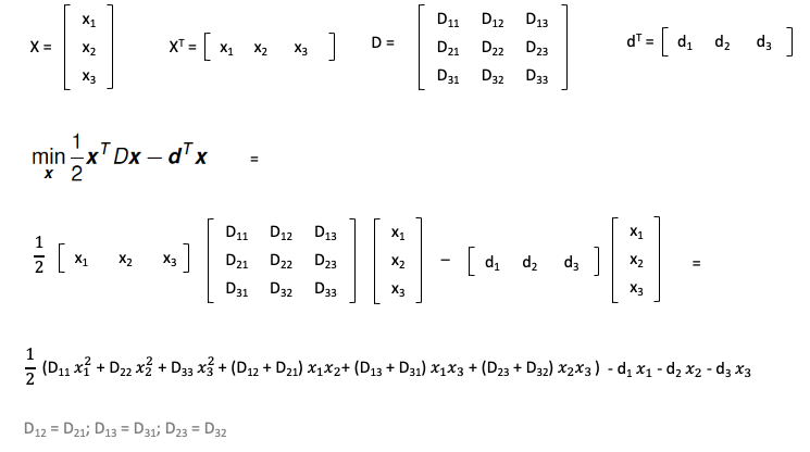
First, let’s consider a general matrix notation for three variables: x₁, x₂, x₃:

Second, the matrix of D and the vector of d can be found by the parameter mapping to the example:

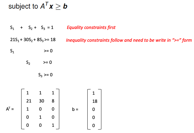
Similarly, the constraint matrix can be found as follows:

Please note that, for the constraints matrix, we need to put equality constraints first and rewrite inequality constraints in “>=” form.

Package quadprog Usage

solve.QP(Dmat, dvec, Amat, bvec, meq=0, factorized=FALSE)

- Dmat    
matrix appearing in the quadratic function to be minimized.

- dvec    
vector appearing in the quadratic function to be minimized.

- Amat    
matrix defining the constraints under which we want to minimize the quadratic function.

- bvec    
vector holding the values of b_0 (defaults to zero).

- meq    
the first meq constraints are treated as equality constraints, all further as inequality constraints (defaults to 0).

- factorized    
logical flag: if TRUE, then we are passing R^(-1) (where D = R^T R) instead of the matrix D in the argument Dmat.

Code & Output

# Load "quadprog" package
# library(quadprog)

# Matrix appearing in the quadratic function
Dmat <- matrix(c(0.125, 0.08, -0.01, 0.08, 0.405, -0.02, -0.01, -0.02, 0.005), 3, 3)

# Vector appearing in the quadratic function
dvec <- c(0, 0, 0)

# Matrix defining the constraints
Amat <- t(matrix(c(1, 21, 1, 0, 0, 1, 30, 0, 1, 0, 1, 8, 0, 0, 1), 5, 3))

# Vector holding the value of b_0
bvec <- c(1, 18, 0, 0, 0)

# meq indicates how many constraints are equality 
# Only the first constraint is equality so meq = 1
qp <- solve.QP(Dmat, dvec, Amat, bvec, meq = 1)
qp

$solution
[1] 0.4019549 0.2170267 0.3810185

$value
[1] 0.02379223

$unconstrained.solution
[1] 0 0 0

$iterations
[1] 3 0

$Lagrangian
[1] -0.049686557  0.005403946  0.000000000  0.000000000  0.000000000

$iact
[1] 1 2

As you can see, the portfolio selection of these three stocks should be qp$solution (40.2% Stock1, 21.7% Stock2, and 38.1% Stock3) and the total risk is $qp$value, 2.4%.

Looking for an example of two variables (x₁ and x₂)? Please also check my another post: Another Quadratic Programming Example with R.