I have been exploring a couple of marketing platforms in my new job as a Marketing Analyst. One of the daily jobs which I like most is to use R to dig into data across different marketing channels to come up with new ideas and recommendations for our marketing activities.
Table of Contents
Google Search Console
Google Search Console is one of the platforms I have been playing with recently. As you may already know, Google Search Console is a useful website tool for marketers to check website overall performance (e.g., search engine crawl and index issues, google search performance). For example, here is the performance report for my personal blog:
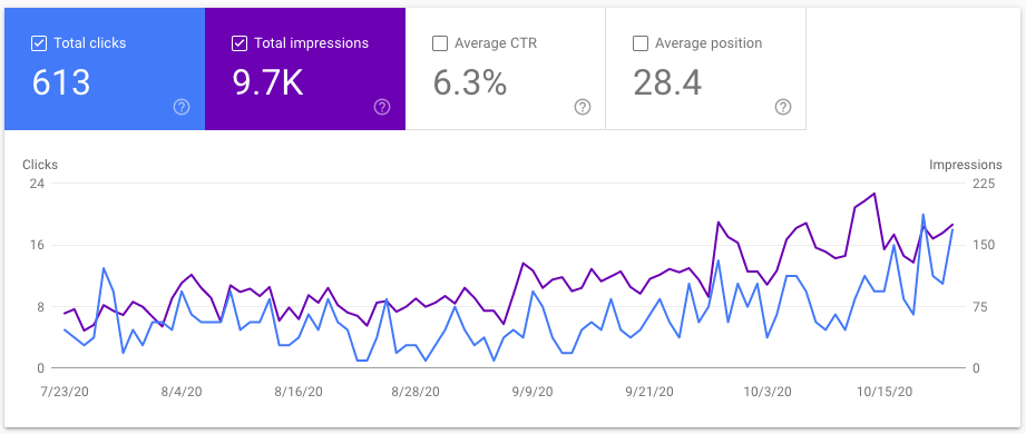
Google Search Performance report for my blog
As you can see from the report, my blog has an average position of 28.4 on the search results, with a gradual increase in terms of impressions and clicks in the past 3 months.
Besides the overall performance report, Google Search Console also provides detailed information for different dimensions, such as query, page and country etc.
searchConsoleR Package
searchConsoleR is the r package I’m using to work with Google Search Console data. It is developed by Mark Edmondson, who also developed a bunch of other Google related r packages such as googleAnalyticsR. Highly recommend to check out his work if you want to do marketing analytics with R.
Pull Data from Google Search Console
I mainly use search_analytics() function in searchConsoleR to access my Google Search Console.
Firt load the packages:
Get the query data in the last 3 months (by default):
# authentication
scr_auth()

query <- search_analytics(
  siteURL = "https://henrywang.nl/",
  dimensions = "query"
) %>%
  as_tibble()

query %>%
  head(10)
#> # A tibble: 10 x 5
#> query clicks impressions ctr position
#> <chr> <int> <int> <dbl> <dbl>
#> 1 quadratic programming in r 44 162 0.272 2.44
#> 2 quadratic programming r 26 105 0.248 2.50
#> 3 media mix modeling in r 21 63 0.333 3.97
#> 4 r quadratic programming 18 93 0.194 4.08
#> 5 marketing mix modeling in r 14 75 0.187 8.32
#> 6 quadprog in r 4 53 0.0755 7.74
#> 7 kindle vocabulary builder export 3 87 0.0345 8.34
#> 8 quadratic optimization in r 3 41 0.0732 6.05
#> 9 assignment problem in r 2 3 0.667 2
#> 10 ggplot theme elements 2 134 0.0149 5.61Get the page data:
page <- search_analytics(
  siteURL = "https://henrywang.nl/",
  dimensions = "query"
) %>%
  as_tibble()

page %>%
  head(10)
#> # A tibble: 10 x 5
#> page clicks impressions ctr position
#> <chr> <int> <int> <dbl> <dbl>
#> 1 https://henrywang.nl/quadratic-programmin… 223 1718 0.130 10.2
#> 2 https://henrywang.nl/transportation-and-a… 149 1076 0.138 20.5
#> 3 https://henrywang.nl/media-mix-modeling-i… 120 2125 0.0565 38.7
#> 4 https://henrywang.nl/kindle-vocabulary-bu… 30 705 0.0426 21.4
#> 5 https://henrywang.nl/maximum-flow-problem… 22 356 0.0618 39.3
#> 6 https://henrywang.nl/ggplot2-theme-elemen… 21 2093 0.0100 26.5
#> 7 https://henrywang.nl/category/optimizatio… 13 111 0.117 19.4
#> 8 https://henrywang.nl/linear-programming-w… 5 293 0.0171 33.9
#> 9 https://henrywang.nl/mediation-analysis-i… 4 342 0.0117 52.1
#> 10 https://henrywang.nl/ 2 60 0.0333 16.9Get query data for each page (answer questions like which keyword is driving traffic to one specific page?):
page_query <- search_analytics(
  siteURL = "https://henrywang.nl/",
  dimensions = "query"
) %>%
  as_tibble() %>%
  group_by(page) %>%
  arrange(desc(impressions)) %>%

page_query %>%
  head(10)
#> # A tibble: 10 x 6
#> # Groups: page [5]
#> page query clicks impressions ctr position
#> <chr> <chr> <int> <int> <dbl> <dbl>
#> 1 https://henrywang.nl/media-… media mix m… 0 795 0 47.6
#> 2 https://henrywang.nl/ggplot… ggplot2 the… 1 275 0.00364 37.9
#> 3 https://henrywang.nl/ggplot… ggplot them… 1 248 0.00403 40.6
#> 4 https://henrywang.nl/ggplot… theme ggplot 0 183 0 31.6
#> 5 https://henrywang.nl/quadra… quadratic p… 44 162 0.272 2.44
#> 6 https://henrywang.nl/probab… rbinom in r 0 139 0 79.1
#> 7 https://henrywang.nl/probab… rbinom in r 0 138 0 79.1
#> 8 https://henrywang.nl/ggplot… ggplot them… 2 134 0.0149 5.61
#> 9 https://henrywang.nl/ggplot… ggplot theme 1 129 0.00775 34.9
#> 10 https://henrywang.nl/quadra… quadprog r 2 126 0.0159 9.81Query Performance Analysis
Depends on different marketing objectives, these data can be used in different ways. As suggested by Google, one of the use cases is to identify queries with high impressions but low ctr and then try to improve them. These keywords are important because, for example, my blog is shown quite often for those queries on the search results but people don’t click the link to my blog proportionally.
These keywords can be identified as follows:
query %>%
  # remove queries with very few impressions
  filter(impressions > 20) %>%
  ggplot(aes(ctr, impressions, label = query)) +
  geom_point(alpha = .5, size = .8) +
  geom_text_repel(size = 3) +
  # average impression is around 90
  geom_hline(yintercept = 90, color = "red", linetype = "dotdash") +
  # average ctr is 6%
  geom_vline(xintercept = .06, color = "red", linetype = "dotdash") +
  scale_y_log10() +
  scale_x_continuous(labels = scales::label_percent(accuracy = 1),
                     breaks = seq(0, .3, .05))
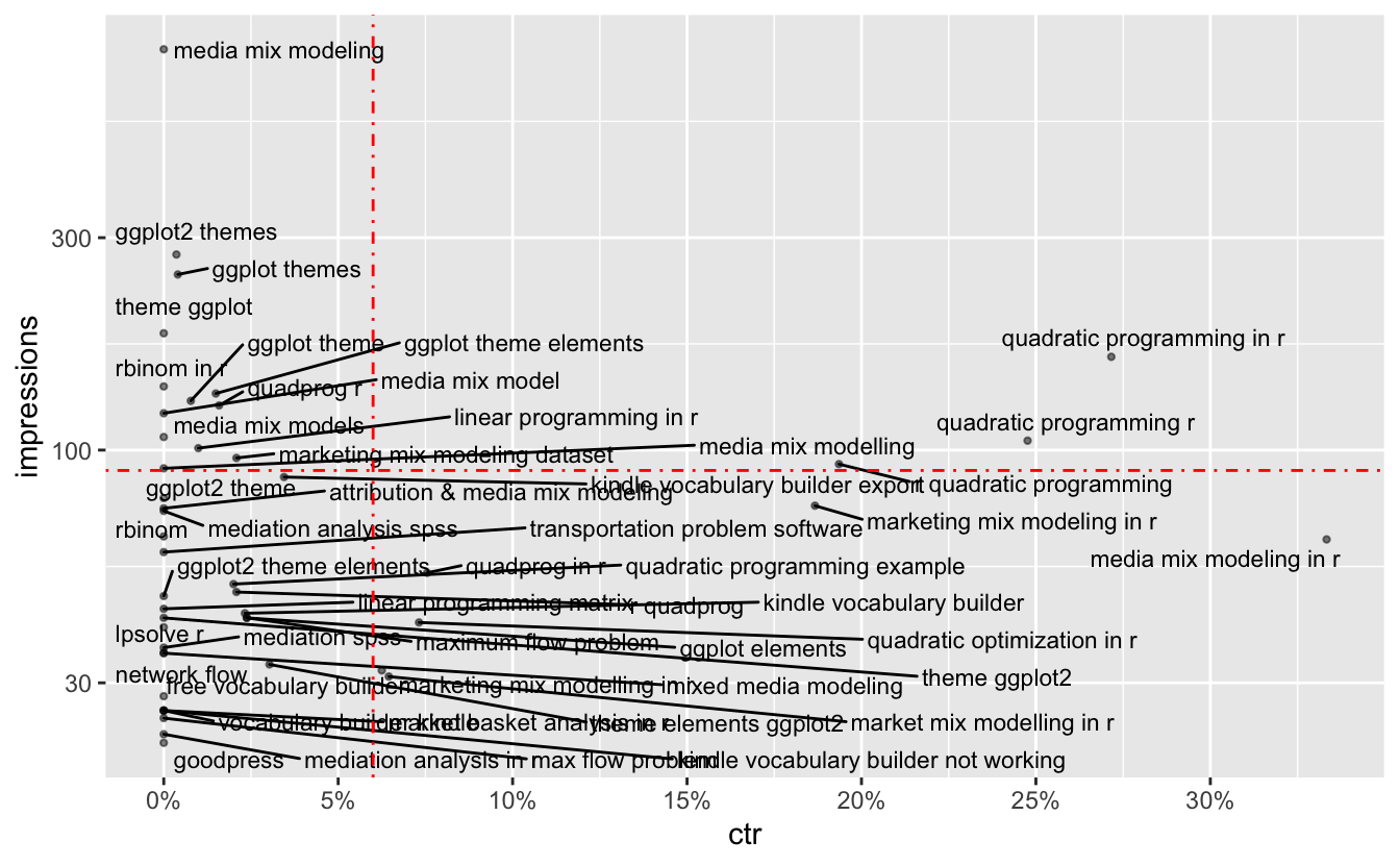
Queries with High Impressions but Low CTR
As you can see from the graph, the top-left grid of the plot shows the queries with high impressions but low ctr, among which are a few keywords (e.g., ggplot2 themes) linked to ggplot2 Theme Elements Demonstration.
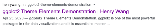
Page Title and Snippet to My Blog on SERP
What I can do next is to improve the page title and meta description to make it more relevant on the search results so that the CTR could be increased, resulting in more traffic to my blog. I didn’t do this for my blog as I don’t want to go that far in that direction but it is highly recommended to implement it for your company website.
This is an example of what we can do with R to conduct marketing analyses. I hope I can share with you more and will keep writing blogs about marketing analysis with R in the next coming weeks!
Hi Henry, great article. What about creating themes of the queries to see if certain themes (like MMM) have a higher overall potential as opposed to individual queries?
Hi Henry, great article.
What about creating themes of the queries to see if certain themes (like MMM) have a higher overall potential as opposed to individual queries?
Just saying because the last graph is a bit difficult to read and deduce from what to do next 🙂
Hi Sara,
Good question! It is possible to group queries in a way as you said during the analysis. Another approach could be using an interactive plot to view individual queries, which I didn’t show in this post.
Thanks!