Table of Contents
Background
In the past few months I have been working on my Master’s Thesis and I just completed the data analysis part, leaving the discussion and conclusion parts. For some reason, this data analysis is conducted in SPSS and I’m always wondering if I could repeat it in R. The topic of my Master’s Thesis is “The influence of IT Capability on New Product Development Performance”. Specifically, my research question is “To what extent does IT Capability relate to NPD Performance and to what extent does NPD Process mediate the relationship?”.
The data was collected with a questionnaire that is designed based on a thorough literature review. After data cleaning, construct validity tests with Exploratory Factor Analysis and construct reliability tests, the latent constructs are computed and the enhanced operational model is presented below:
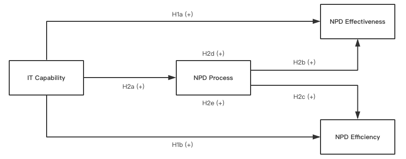
Depicted from the operational conceptual model, NPD Performance is measured by two distinct sub-constructs (NPD Effectiveness and NPD Efficiency). Accordingly, the hypotheses are formulated as follows:
Hypothesis 1a: A higher level of IT Capability leads to a higher level of NPD Effectiveness.
Hypothesis 1b: A higher level of IT Capability leads to a higher level of NPD Efficiency.
Hypothesis 2a: A higher level of IT Capability leads to a higher level of NPD Process.
Hypothesis 2b: A higher level of NPD Process leads to a higher level of NPD Effectiveness.
Hypothesis 2c: A higher level of NPD Process leads to a higher level of NPD Efficiency.
Hypothesis 2d: NPD Process mediates the relationship between IT Capability and NPD Effectiveness.
Hypothesis 2e: NPD Process mediates the relationship between IT Capability and NPD E
Data Analysis Strategy
The analyses are conducted with Model 4 (Figure 2) in

In Model 4, X is modeled to influence Y directly as well as indirectly through a single mediator variable M causally located between X and Y (Hayes, 2012). While the direct effect of X on Y is estimated with c’1, the indirect effect of X on Y through M is estimated as a1b1, meaning the product of the effect of X on M (a1) and the effect of M on Y controlling for X (b1). The direct and indirect effect of X on Y sum to yield the total effect of X on Y (c1), meaning that c1 = c’1 + a1b1. The total effect can also be estimated by the direct effect of X on Y when no mediator is included in the regression.
The mediation exists if there is a significant indirect effect (a1b1). More specifically, partial mediation exists if the direct effect of X on Y remains significant with a significant indirect effect. In turn, full mediation occurs if the direct effect of X on Y is no longer significant with a significant indirect effect. Confidence intervals are used to assess the mediation. There is no evidence of indirect effects if the confidence intervals cross zero.
Basically, the mediation analysis includes the following steps:
- Step 1: Examining the total effect of X on Y, namely c1 in Model 4. In the case of my thesis, this results in hypothesis 1a and 1b are supported or not;
- Step 2: Examining the direct effect of X on M, which is the effect of a1 in Model 4. Hypothesis 2a will be supported or not;
- Step 3: Examining the direct effect of M on Y controlling X, which is b1 in Model 4. Consequently, hypothesis 2b and 2c are supported or not;
- Step 4: Examining the indirect effect of X on Y, which is a1b1, this will find support for hypothesis 2d and 2e or not;
- Step 5: Checking if the direct effect of X on Y is still significant with a significant indirect effect to decide it is a partial or full mediation;
Mediation Analysis in SPSS
Following the instruction above, the mediation analysis in SPSS is quite straightforward and easy. The setup is shown below (Figure 3).

As shown in Figure 3, some control variables are also included
Run MATRIX procedure:
 * PROCESS Procedure for SPSS Beta Release 120212 *
     Written by Andrew F. Hayes, Ph.D.   http:www.afhayes.com

****************************************************************************
 Model = 4
     Y = Effectiv
     X = ITC
     M = IPF
 Statistical Controls:
 CONTROL= Firm_Emp IS_Emplo IS_Age   Industry
 Sample size
         162
****************************************************************************
 Outcome: IPF
 Model Summary
           R       R-sq          F        df1        df2          p
       .6194      .3836    19.4181     5.0000   156.0000      .0000
 Model
               coeff         se          t          p       LLCI       ULCI
 constant     1.2571      .3102     4.0524      .0001      .6443     1.8698
 ITC           .6538      .0674     9.6984      .0000      .5207      .7870
 Firm_Emp     -.0235      .0190    -1.2365      .2181     -.0610      .0140
 IS_Emplo     -.0125      .0241     -.5190      .6045     -.0602      .0351
 IS_Age        .0512      .0381     1.3453      .1805     -.0240      .1264
 Industry      .0052      .0098      .5366      .5923     -.0141      .0245

****************************************************************************
 Outcome: Effectiv
 Model Summary
           R       R-sq          F        df1        df2          p
       .5753      .3310    12.7809     6.0000   155.0000      .0000
 Model
               coeff         se          t          p       LLCI       ULCI
 constant     1.6134      .3055     5.2809      .0000     1.0099     2.2169
 IPF           .2703      .0750     3.6041      .0004      .1222      .4185
 ITC           .3049      .0800     3.8133      .0002      .1470      .4629
 Firm_Emp      .0023      .0179      .1312      .8958     -.0330      .0377
 IS_Emplo     -.0161      .0226     -.7121      .4775     -.0608      .0286
 IS_Age        .0459      .0359     1.2797      .2026     -.0250      .1168
 Industry     -.0044      .0092     -.4856      .6280     -.0225      .0137

*************************** TOTAL EFFECT MODEL *****************************
 Outcome: Effectiv
 Model Summary
           R       R-sq          F        df1        df2          p
       .5243      .2749    11.8300     5.0000   156.0000      .0000
 Model
               coeff         se          t          p       LLCI       ULCI
 constant     1.9532      .3016     6.4769      .0000     1.3575     2.5489
 ITC           .4817      .0655     7.3493      .0000      .3522      .6111
 Firm_Emp     -.0040      .0185     -.2168      .8286     -.0405      .0325
 IS_Emplo     -.0195      .0234     -.8311      .4072     -.0658      .0268
 IS_Age        .0597      .0370     1.6144      .1085     -.0134      .1328
 Industry     -.0030      .0095     -.3191      .7501     -.0218      .0157

***************** TOTAL, DIRECT, AND INDIRECT EFFECTS **********************
 Total effect of X on Y
      Effect         SE          t          p       LLCI       ULCI
       .4817      .0655     7.3493      .0000      .3522      .6111
 Direct effect of X on Y
      Effect         SE          t          p       LLCI       ULCI
       .3049      .0800     3.8133      .0002      .1470      .4629
 Indirect effect of X on Y
         Effect    Boot SE   BootLLCI   BootULCI
 IPF      .1767      .0597      .0730      .3135

******************** ANALYSIS NOTES AND WARNINGS ***************************
 Number of bootstrap samples for bias corrected bootstrap confidence intervals:
      1000
 Level of confidence for all confidence intervals in output:
     95.00
 NOTE: Effect size measures for indirect effects not available for models with covariates
 ------ END MATRIX -----
We could interpret the result above following the instructions (please note that in the output ITC = IT Capability, IPF = NPD Process, Effectiv = NPD Effectiveness).
Step 1: Examining the total effect of X on Y
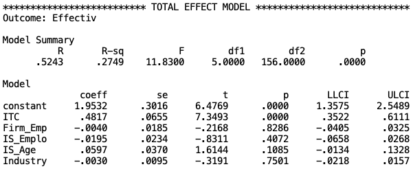
With R-square = .2749 and F-statistic = 11.8300 (p < .001), this model is significant. Furthermore,
Step 2: Examining the direct effect of X on M
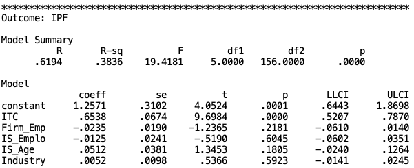
Similarly, IT Capability is significantly positively related to NPD Process. Hypothesis 2a is supported.
Step 3: Examining the direct effect of M on Y controlling X
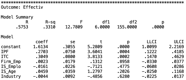
NPD Process is significantly positively related to NPD Effectiveness. Hypothesis 2b is supported.
Step 4: Examining the indirect effect of X on Y
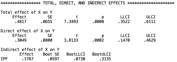
As shown in Figure 7, the indirect effect of IT Capability on NPD Effectiveness is significant (LLCI = .0730, ULCI = .3135). Hypothesis 2d is supported.
Step 5: Checking if the direct effect of X on Y is still significant
Also as shown in Figure 7, the direct effect of IT Capability on NPD Effectiveness is still significant (LLCI = .1470, ULCI = .4629) with a significant indirect effect (Step 4), so it is a partial mediation. In conclude, NPD Process partially mediates the relationship between IT Capability and NPD Effectiveness.
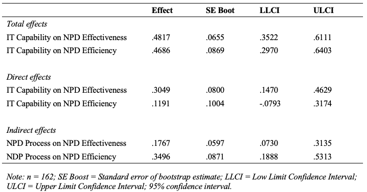
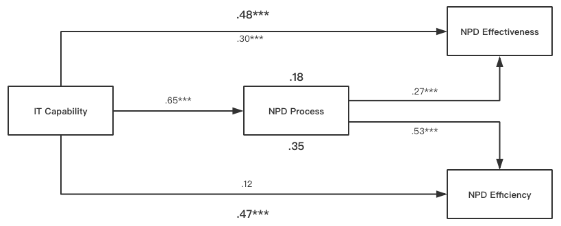
The mediation analysis can be run for another dependent variable (NPD Efficiency) similarly. The final results can be reported in the thesis as below (Figure 8 and Figure 9).
Mediation Analysis in R
Using the same mediation analysis strategy, the analysis in R is similar.
# Loading data from local directory
load("thesis.RData")
# Loading "psych" package to use "mediate" function
library(psych)
# Run "mediate" function
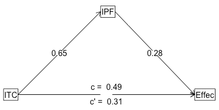
mediation <- mediate(Effec ~ ITC + (IPF), data = thesis, plot = TRUE, n.iter = 1000)
# Plot the result
mediation
# The longer output
summary(mediation)
Here are the output and plot.
Call: mediate(y = Effec ~ ITC + (IPF), data = thesis, n.iter = 1000,
     plot = TRUE)

Total effect estimates (c)
     Effec   se   t  df     Prob
 ITC  0.49 0.06 7.5 159 4.12e-12

Direct effect estimates     (c')
     Effec   se    t  df     Prob
 ITC  0.31 0.08 3.90 159 0.000142
 IPF  0.28 0.07 3.76 159 0.000236

 R = 0.57 R2 = 0.32   F = 37.56 on 2 and 159 DF   p-value:  4.38e-14

 'a'  effect estimates
      IPF   se    t  df     Prob
 ITC 0.65 0.07 9.72 160 7.88e-18

 'b'  effect estimates
     Effec   se    t  df     Prob
 IPF  0.28 0.07 3.76 159 0.000236

 'ab'  effect estimates
     Effec boot   sd lower upper
 ITC  0.18 0.18 0.06  0.07  0.28
Since I didn’t include control variables, the final result was slightly different.
The package I’m using is “psych”, while there is another one called “mediation”. Furthermore,
References:
Hayes, A. F. (2012). PROCESS: A versatile computational tool for observed variable mediation, moderation, and conditional process modeling.
BWER Company provides Iraq’s leading-edge weighbridge solutions, designed to withstand harsh environments while delivering top-tier performance and accuracy.