While attribution measurements are widely used in the digital marketing field, Media Mix Modeling (MMM) still plays an important role in evaluating marketing effectiveness across multiple channels at a higher level. Here is an example of how to do MMM in R with a free dataset from Kaggle.

Data Preparation

library(tidyverse)

# Import data
media.raw <- read_csv("mediamix.csv")

# Tidy data
media <- media.raw %>%
      mutate(TV = tv_sponsorships + tv_cricket + tv_RON) %>%
      mutate(Digital = rowSums(.[9:13])) %>%
      select(TV, radio, Magazines, OOH, Digital, sales) %>%
      rename(Radio = radio, Sales = sales)

# Examining data
View(media)

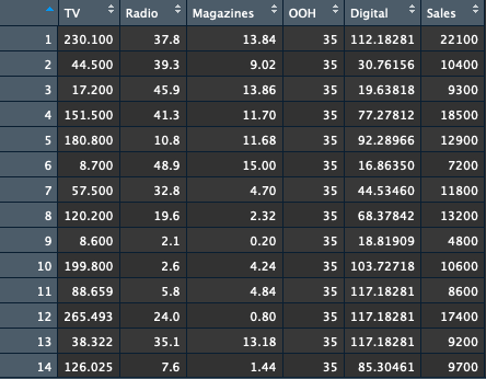
Three TV-related channels are combined as TV variable. Similarly, the Digital variable is computed from channels such as Social, Display, Search, etc. The final data structure is shown as follows. This article is to examine the relationship between the dependent variable of Sales and the independent variables of TV, Radio, Magazines, OOH, and Digital. The numbers represent the media cost across channels.

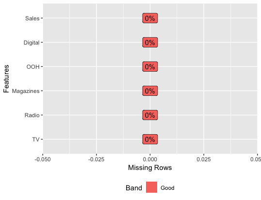
Furthermore, there is no missing value in the dataset.

# Checking missing values
library(DataExplorer)
plot_missing(media)

Regression Analysis

Before regression modeling, a correlation analysis is conducted to check the potential multicollinearity issue.

# Correlations
library(corrplot)
library(gplots)
corrplot.mixed(corr = cor(media, use = "complete.obs"),
               upper = "ellipse", tl.pos = "lt",
               upper.col = colorpanel(50, "red", "gray60", "blue4"))

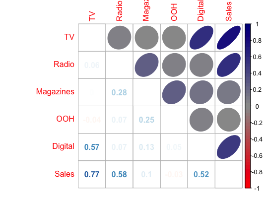
As shown in the correlation matrix, the correlations among the independent variables (e.g., TV, Radio, Magazines, OOH, and Digital) are all below 0.7, so there is no multicollinearity issue. In addition, Sales seems to be highly correlated with TV, and moderately correlated with Radio and Digital based on the preliminary analysis.

Following correlation analysis, the multiple regression analysis is performed first with all the independent variables, then without OOH, of which the coefficient is not significant.

# Regression modeling with all the independent variables
lm1 <- lm(Sales ~ ., data = media)
summary(lm1)

# Regression modeling without OOH
lm2 <- lm(Sales ~ TV + Radio + Magazines + Digital, data = media)
summary(lm2)

# Comparing Models
summary(lm1)$r.squared
summary(lm2)$r.squared

Based on the final results of the regression analysis, the linear equation can be approximately denoted by:

Sales = 39.48*TV + 193.39*Radio – 84.85*Magazine + 12.39*Digital + 2916.41

It can be interpreted as follows:

(1) If no media expenditure spent on advertising, there will be around 2916 sales, which comes from organic traffic;

(2) The priority of the media channels should be Radio > TV > Digital, according to their coefficients. For example, let’s suppose the numbers in the media cost in this dataset is in $1000 unit, then an additional $1000 spent on Radio could increase around 193 additional sales;

(3) Magazine has a negative effect on Sales and therefore should be paused if possible.