Probability in R | Henry Wang

I can still remember the nightmare when I first studied Statistics in my Bachelor a few years ago. It was a nightmare because we were asked to do all the exercises and exams on paper without cheat sheets and even calculators. However, the Statistics course in my Master turned out much more interesting as all the exercises and exams were conducted online and we were allowed to use Excel formulas as well. A couple of days ago when I came across Foundations of Probability in R on DataCamp I realized that learning statistics could be much better with random simulation and data visualization in R. This course is quite fundamental and nothing new to me but the idea behind it is very appealing.

Table of Contents

Binomial Distribution

Let’s say I’m flipping a fair coin (50% chance of “heads” and 50% chance of “tails”) 10 times in an experiment, how many “heads” I will end up with?

If lucky, I may have 10 “heads” at most, or on the other hand, I don’t have any “heads” at all, but most likely it is in between. Let’s suppose the number of “heads” (X) is 4 at my first try.

What if I repeat this experiment 100000 times? I will definitely get 100000 values of X and as we can see later, the number of “heads” (X) follows a binomial distribution.

Random Simulation with rbinom()

If each experiment (flipping a coin 10 times and record the number of “heads”) takes me 1 minute, the 100000 experiments maybe would take me approximately 1667 hours to complete! In contrast, this can be easily simulated in seconds in R.

# rbinom(observations, trials, probability)
# probability: the probability of success in each trial
# return value: the number of success trails in each observation, discrete value

flips <- rbinom(100000, 10, 0.5)

Density Probability with dbinom()

If I flip a fair coin 10 times, what is the probability that I end up with 5 “heads”, Pr( X = 5)? This can be answered in two different ways.

# Method 1: approximate probability with simulation
mean(flips == 5)

# Method 2: exact probability with dbinom()
dbinom(5, 10, 0.5)

Cummulative Density with pbinom()

Similarly, the probability that the number of “heads” less than 5, Pr( X <= 5), can be calculated as follows.

# Method 1: approximate probability with simulation
mean(flips <= 5)

# Method 2: exact probability with dbinom()
pbinom(5, 10, 0.5)

Binomial Distribution Visualization

library(tidyverse)
library(patchwork)

# Data preparation
flips_viz <- tibble(heads = factor(flips)) %>%
      count(heads, name = "count") %>%
      mutate(dbinom = count / sum(count), pbinom = cumsum(dbinom))

# Frequency visulization, rbinom()
p1 <- ggplot(flips_viz, aes(heads, count)) +
      geom_col() +
      ylab("Frequency")

# Density visulization, dbinom()
p2 <- ggplot(flips_viz, aes(heads, dbinom)) +
      geom_point() +
      geom_line(group = 1) +
      ylab("Density")

# Cummulative Density visualization, pbinom()
p3 <- ggplot(flips_viz, aes(heads, pbinom)) +
      geom_point() +
      geom_line(group = 1) +
      ylab("Cummulative Density")

# Combine into one plot
p1 + p2 + p3

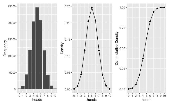
As shown in the graph, 5 “heads” appeared the most, followed by 4 “heads” and 6 “heads”. Apparently, in this way Binomial distribution can be easily understood and the principles behind can be applied to other distributions.

Normal distribution

Simulating from binomial distribution to normal distribution: flipping a coin many times, 1000 times in each experiment in this example.

# Binomial distribution
binomial <- rbinom(100000, 1000, .5)
expected_value <- 1000 * .5
variance <- 1000 * .5 * (1 - .5)
sd <- sqrt(variance)

# Normal distribution
# rnorm(observations, mean, sd)
# mean: how is the data-centered?
# sd: how is the data spread
# return value: random deviates with mean and sd, continous value
normal <- rnorm(100000, expected_value, sd)

# Comparison
tibble(binomial = binomial, normal = normal) %>%
      pivot_longer(cols = everything(), names_to = "dist", values_to = "heads") %>%
      ggplot(aes(heads)) +
      geom_histogram() +
      facet_wrap(~dist, ncol = 1)

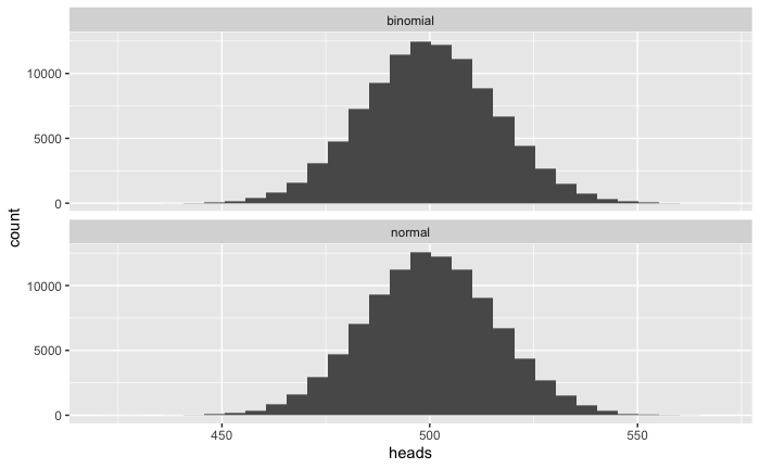
As shown above, as flipping the coin many times in each experiment binomial distribution is very similar to normal distribution.

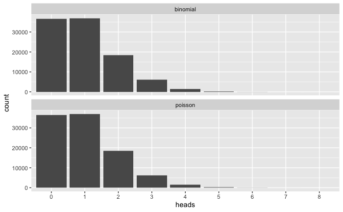
Poisson Distribution

Simulating from binomial to Poisson: flipping a coin many times, each with a very low probability of “heads”.

# Binomial distribution
bi_poisson <- rbinom(100000, 1000, 1 / 1000)

# Poisson distribution
# rpois(observations, lambda
# expected value = lambda, approximately equals to expected value of   # binomial distribution, np
# variance = lambda
# return value: random deviates with lambda, discrete value
poisson <- rpois(100000, 1)

# Comparison
tibble(binomial = bi_poisson, poisson = poisson) %>%
      pivot_longer(cols = everything(), names_to = "dist", values_to = "heads") %>%
      ggplot(aes(factor(heads))) +
      geom_bar() +
      scale_x_discrete("heads") +
      facet_wrap(~dist, ncol = 1)

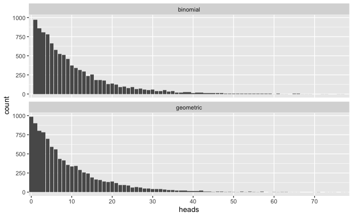
Geometric Distribution

How many times does it take me to flip a coin to get a “heads”?

# Simulating from binomial to geometric
bi_geom <- replicate(10000, which(rbinom(100, 1, .1) == 1)[1])

# Geometric distribution
rgeom(observations, probability)
geom <- rgeom(10000, .1)

# Comparison
tibble(binomial = bi_geom, geometric = geom) %>%
      pivot_longer(cols = everything(), names_to = "dist", values_to = "heads") %>%
      ggplot(aes(factor(heads))) +
      geom_bar() +
      scale_x_discrete("heads", breaks = c(0, 10, 20, 30, 40, 50, 60, 70)) +
      facet_wrap(~dist, ncol = 1)